Calculating Running Totals and Temporal Trends in MongoDB

The Fundamental Change in Document Analytics

Until recently, document databases have only been considered as high-speed databases by developers and architects. Relational database systems have been ruling the complexity of reporting, analysis, and time calculations so that when an engineering team needed run rates, moving average, rank distribution, period-on-period variance, etc., MongoDB was considered only at the extraction stage. Later, data was either transported to the data warehouse or processed in the middle of other applications written in Java, Python, or Node.js.

The introduction of the windowing function in the aggregation stage has changed all that. Now, instead of making numerous costly collection scans, performing self-joins, manipulating array unwinds, and developing complicated multi-thread MapReduce logic, it is now possible to calculate all the metrics in one database engine stage.

Understanding how to master the use of window functions allows us to carry out sophisticated processes related to data analysis, time-series analysis, supply chain analysis, and analysis of user activities in MongoDB. If you want to develop your experience in creating the aforementioned pipelines, you can attend a specialized training that teaches how to go beyond basic queries using a mongodb course. Post-processing can also become more advanced as a result of removing any network delays and delays in computation associated with transferring data from the database to the to-be-analyzed backend.

Understanding the Core Architecture of Window Functions

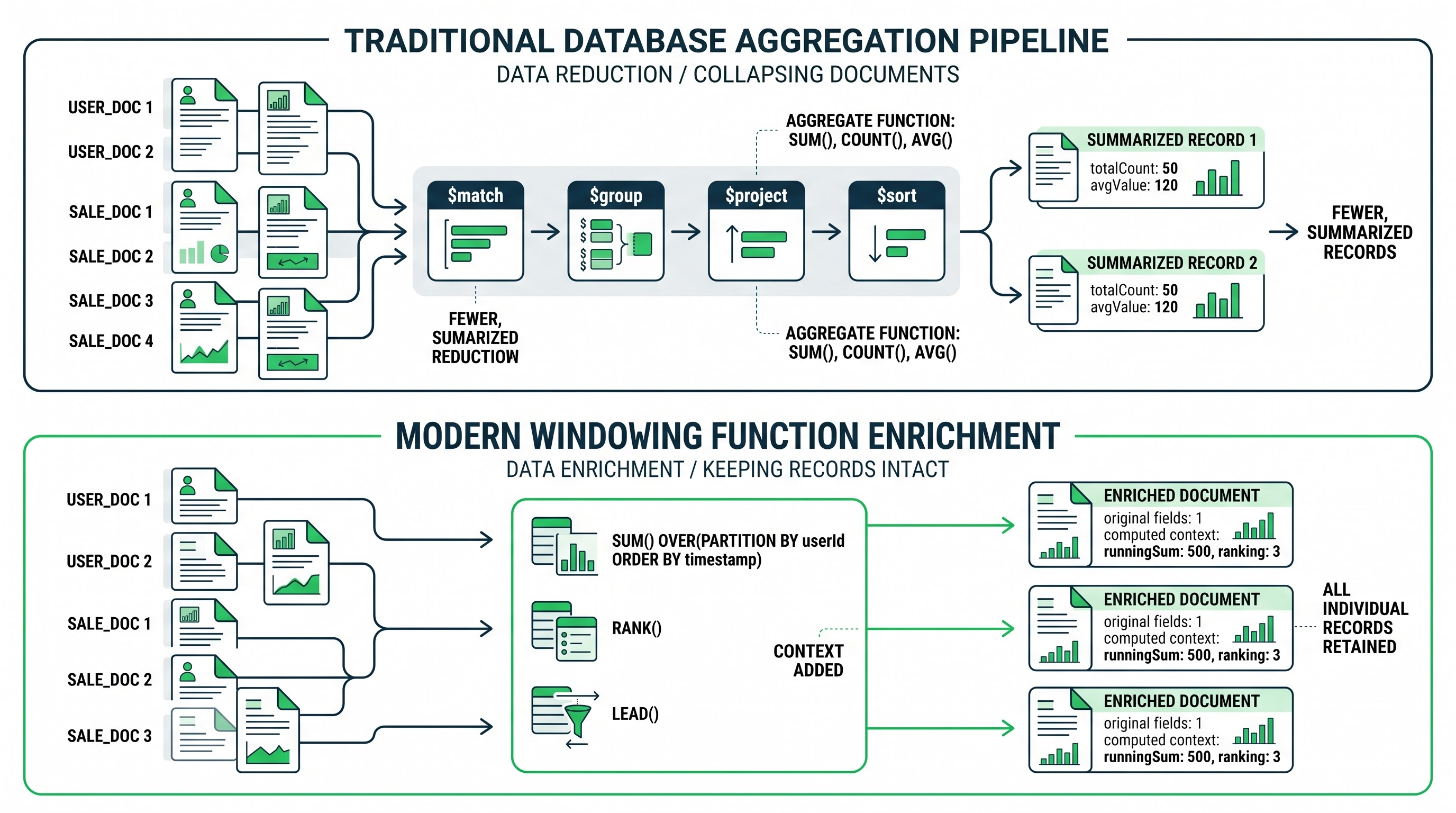
The first step in understanding the benefits of window functions is comparing them to traditional ways of group processing. In a typical aggregation process, the stage of grouping serves as a filtering process. When there are millions of transactions among many categories in the database, the group function reduces the number of documents in the collection to one document per category and allows computing total sales or total quantity sold but eliminates any record identity of the documents that are used in the process.

Window functions function on a completely different plane of thought than the regular operations because rather than aggregating several rows into one, a window function performs an action on several records but keeps all records intact in the data pipeline. When results are generated, every record gets processed, but it gets the results calculated based on nearby records and goes further.

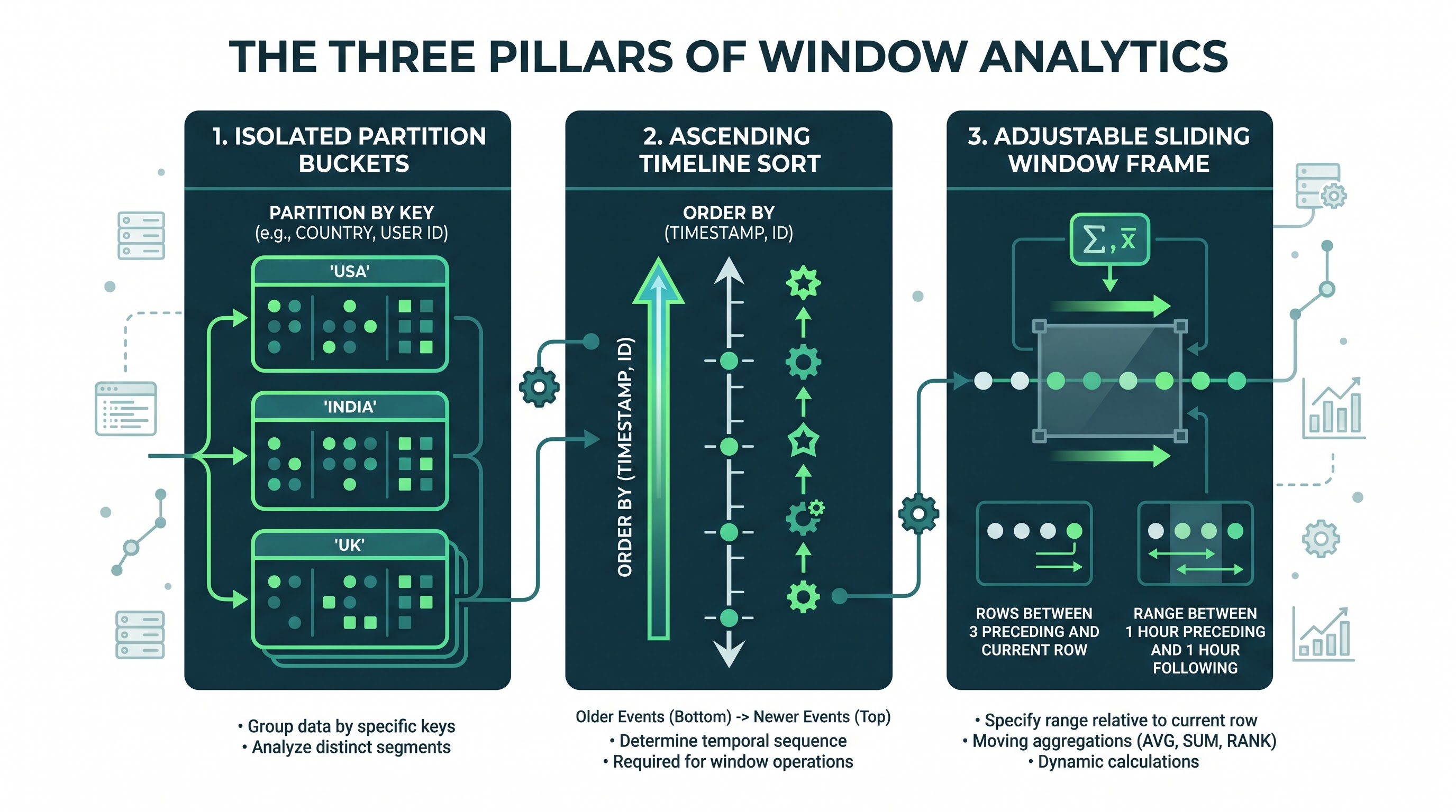
To make this possible, there are three parts that create the foundation of window functions: partitioning, sorting, and definition of the frame.

Partitioning the Dataset

Partitioning the dataset refers to the process of establishing the limits. Partitioning limits documents into subsets that do not communicate with each other. For example, in a situation of analyzing financial transactions, one may create partitions by accounts used to conduct the transactions. In the case of monitoring the server telemetry, the name of the host or the region of the datacenter may serve as a key used to create partitions.

Calculations happening within any partition have no connection to other partitions. Whatever total for Account A is calculated, this will have nothing to do with Account B. An absence of any partition expression will mean that the system will consider all the incoming data as a universal partition. Thanks to this separation, the aggregation engine operates in a very efficient way, keeping its processing organized by tracking the states along each partition’s borders.

The Vital Importance of Sorting

Calculations that are concerned with running totals and averages are directional and temporal in nature as they depend solely on the sequence. Assuming that there is no known sorting order it is impossible to understand the meaning of measures like previous transactions, previous week, or next temperature record.

Sorting in the windowing stage will ensure that all documents in all partitions will now be arranged in a certain sequence as determined by the sorting logic. Most often, this sorting key is a timestamp, an auto-incrementing serial or a number that keeps temporal sequence. After all documents are sorted, the engine will be able to determine the documents that were in front of and behind the document that was currently being processed.

The concept of the Window Frame

Window frame describes how far one can consider neighboring documents for calculating the output field in the current document. Document frames can be based on two approaches: document-based framing and range-based framing.

In a document-based frame, the start and end of a frame are determined based on certain offsets from the current document position in the sorted partition. For instance, a frame may say that two preceding records and the current document will be included in the evaluation. This method exclusively depends on positions as it does not take into account the time interfere between records but only the number of documents.

On the other side, a frame that uses a specific range of values sets parameters for the time period being examined. This is necessary for real-life time-series data where the frequency of reporting intervals is variable. Sensor malfunction, network problems, and fluctuations in user load lead to missing records. For example, in the case of a range-based frame, one such value might be all records containing timestamps within seven days of the current one. Even if three out of seven days had no records, a range-based frame successfully handles that gap, whereas a document-based frame would include older records from the past timeframe mistakenly.

The edges of the window frame may also be specified as unbounded. An unbounded lower edge tells the engine to go all the way back to the beginning of the partition, while an unbounded upper edge counts forward to the end of the series. By manipulating the positions of the upper edge, the lower edge, and the existing position in the window, developers can create extending, entering, and centered windows based on requirements for the analytical task.

Calculation of Rolling Total and Cumulative Aggregates

Rolling total is the most used cumulative calculation in the corporate sector. It answers questions about total income received at a certain time, total expenses for marketing during one campaign, depletion of stocks during a sales period, and total data consumed on the cloud web server.

The process involved in cumulative accumulation

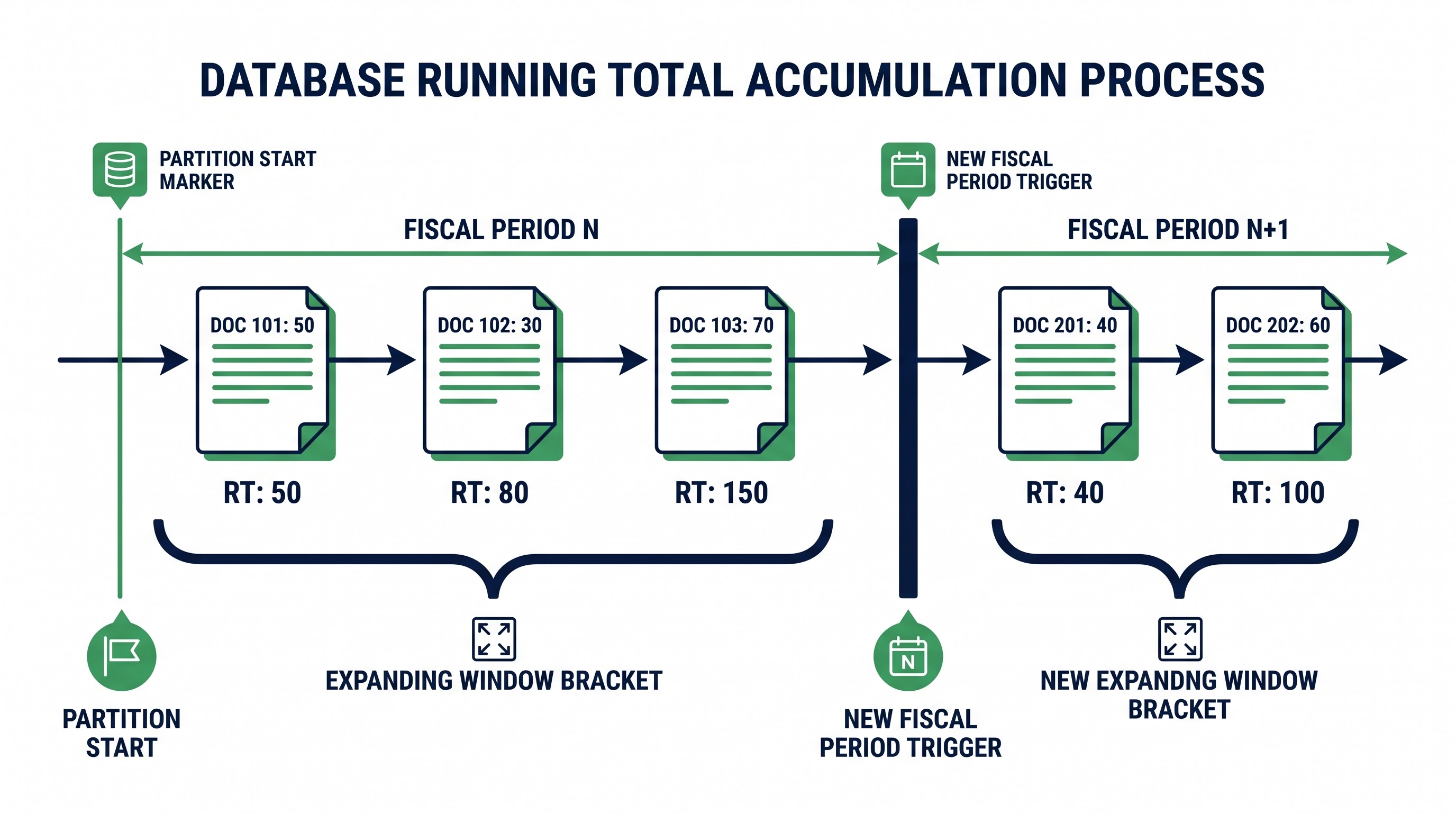
In the process of determining a running total, the system begins its work from the first data available in a partition and creates a running accumulator. In terms of the first data record, the corresponding cumulative total is equivalent to this particular record's value. The engine proceeds to accumulate values from each new record being added to the system.

To achieve a reliable running total, a window frame must be created with a lower limit that is not restricted by anything and an upper limit that represents the current record only. The structure thus created is known as an expanding window since while the evaluation pointer is moving through the records, the window's size keeps increasing behind the pointer and thus remains always comprehensive.

If, by mistake, we set up an unbounded upper boundary instead, then the engine will derive a grand total for the entire partition and will apply the same grand total to each document in the partition. While this is beneficial for percentage-of-total calculations, it makes the running total lose its ability to deliver a progressive narrative.

Resetting boundaries and multi-tenancy

Due to the nature of multi-tenancy, data of many independent clients/tenants exists in the same physical collection. Thus, running total for one client cannot affect the historical balance of another client.

At this point, the partition key is essential because it creates virtual compute tracks with the help of customer identifier or tenant key in MongoDB. After the pipeline finishes working on the last record for customer A, it resets its accumulator back to zero and starts working on the first document for client B.

Additionally, the running totals must regularly reset within a given entity. For example, when accounting data is recorded in ledgers, the balances are accumulated year to date and should be cleared starting the first day of the fiscal year. If the composite partition key consists of the account number and the year, partitions will be created automatically. The year turnover automatically switches the partition. The recorded values will be captured from January 1st so that there is no need to apply any programming logic or engage in any post-cleaning operations. By learning these multi-tenant partitioning methods and complex pipeline stages, students in profession-oriented mongodb classes will learn some key techniques that will help them function as engineers capable of solving large-scale business tasks without failure.

Creating Moving Averages for Noise Minimization

Raw time series data is hardly ever pure and unambiguous. The e-commerce website traffic goes up in the evening and drops in the morning; the processor makes quite a few unsuccessful calculations; the business revenue changes throughout the week. As a result, at some point, the manager is trying to identify some more or less stable signals amidst the randomly changing telemetry data.

Moving averages is the name given to the most important technique employed in the smoothing process. By making numerous calculations based on a series of values over a given period, loss and surges will come to cancel each other in the process of evaluating the true speed of movement.

Positional moving average: the fixed number method

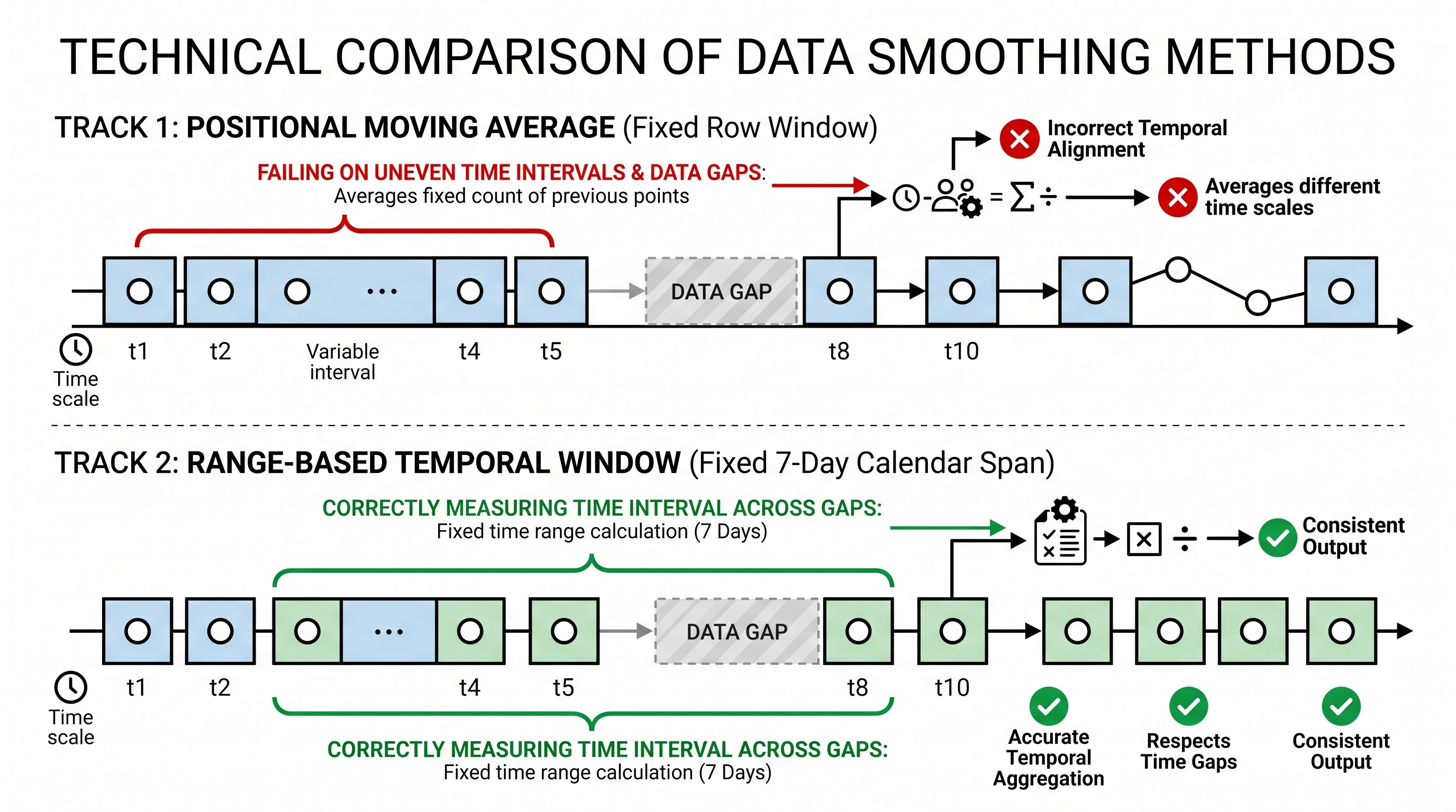
The easiest way of making the use of the moving average is called positional moving average. In this case, the window determines the number of adjacent records. For instance, the simple moving average consists of three records: record number n, one of them preceding and and one following it.

Another aspect of trailing moving averages is their applicability to real-time forecasting scenarios, since the windowing, in this case, evaluates not only presence of the current document but also history of a certain amount of documents. For example, to obtain the average page speed for the last twenty requests, the achieved results become less noisy in a minute without further documentation to wait for.

However, textual moving averages are subject to an important flaw—requirements for constant equidistant observation. Using a temperature gauge providing readings every ten seconds when everything works fine, one would get a moving average of six records for one minute rolling average computed. But if a sensor does not work for five hours before restarting and subsequently provides six readings within the first minute of its work, positional six-record average would not take such a break into consideration while calculating the value.

Moving Averages Based on Periods

Using a range-based approach allows the developer to dissociate the document count from the window frame and connect it with the time elapsing from the sort field. For example, for a seven-day moving average of daily sales, the "window frame" does not consist of seven documents, but rather represents an explicit period of time equal to seven days prior to the document's date.

In the case of application of the temporal window, the database engine first looks at the timestamp of the document and then moves back along the timeline of the partition and gets all the documents that fall into the specific time period defined by the window frame. Therefore, if the e-commerce site has no sales on Tuesday and Wednesday, the moving average for Wednesday involves document records from the previous Friday to Monday without distortions of the value of the period.

The approach is crucial for determining the classical financial metrics of thirty day moving averages for stock volatility, rolling ninety day churn rates for subscriptions and rolling fifteen minute error rates in distributed microservices.

Quantifying Time-Over-Time Trends and Period Deltas

Gathering overall progress is important and removing noise is also significant; however, most enterprise analytics is based on the analysis of deltas – making a comparison between the current state and previous states. Neither business executives ask only about the amount of revenue earned today; they usually want to know whether today’s revenue is higher or lower than yesterday’s, how this month’s performance compares with the same month in the previous year, and what the pace of gaining new customers has been like.

The windowing operators offer customized navigation tools to access data from the nearby or distant documents of the partition without altering the configuration of the pipeline stream.

Utilizing Relative Offsets

Relative offset operators allow looking back and forward in the document stream without interruption. The necessary operator for comparing history is the operator which retrieves the field value from the document located a certain number of steps ahead of the current one. The operator which looks forward is used when looking through documents located a certain number of steps behind the present document.

For instance, in a daily production log, shifts of defects must know the number of defects from the previous day to determine shifts of the defects. Thanks to an offset operator, with a step of one, an offset is applied to the new document from the last day so subtractions show the difference between the two days.

Since each document is processed independently, it is possible to simultaneously calculate absolute variances and proportional growth rates. The stream will take the current day's actual value and compare it to the projection for the preceding day, allowing the stream to determine whether the increase amounted to five units or fifty percent of the value of the metric, which consequently makes it possible for downstream dashboards to instantly signal any violation of critical thresholds.

Calculating Year-On-Year and Quarter-On-Quarter Changes

While one-day and week-by-week assessments involve the use of a short-term sequential approach, measuring seasonal and macroeconomic trends relies on a longer time metric. The industries of retail, hospitality, and agriculture are the ones to confirm that week-to-week analysis may not provide much benefit due to the seasonal cyclic nature of the industries. The income of the skiing resort will be extremely low in July compared to January, so comparing July with June will not provide much useful information either.

To implement this in MongoDB, one can opt for either wide positional offsets or calendar-aligned composite keys.

If the database offers uniformly perfect and complete daily reporting, then a data point can be compared to its counterpart from a year ago simply by looking back exactly 365 positions in the dataset. This method may work in theory, although in practice it is likely to fail due to countless factors. A leap year or daylight saving time may cause the position counter to fail and assess Tuesday against Monday, or some date in August against late July.

In this case, the preferred approach is organizing the partitioning strategy or applying date arithmetic in time windows. In fact, it is possible to calculate the moving average for 30-day windows across similar historical months or use range frames covering the previous year to obtain reliable year-over-year deltas.

Document Ranking and Distribution Analysis

In addition to time-sensitive tracking and tracking trends, data applications of today need advanced distribution analyses. Organizations often require ranking items within competitive categories, classifying transactions by means of percentiles, and establishing which entities perform best across locations.

Dense Ranking versus Standard Ranking

The traditional sorting of documents has presented records in descending order of revenue. However, customary sorting does not generate ordinal ranks even though some applications use it to display rankings of records instead of producing ranks.

It is crucial to make clear the difference between two types of ranking: standard and dense ranking.

Standard ranking, as the name implies, ranks the items based on certain criteria and assigns a rank number to them throughout the sequence. In cases of tied ranks, standard ranking gives the same rank to both tied items but skips subsequent ranks in the sequence according to the number of ties. For instance, if two salesmen are tied in second place, they will earn the rank of two, but the subsequently ranked item will receive a rank of four. Rank three would not exist in this case.

Dense ranking means the same rank is given to tied items, but no gaps are created in the rankings of subsequent items. For example, when two items rank in second place, the next item will receive a rank of three. Dense ranking is widely used in gamification systems, educational fields, and loyalty reward systems where rank gaps may create difficulties for users.

Percentile Bucketing and Quartiles

In massive datasets containing millions of documents, it isn’t useful to simply rank each document in integers. A customer with a ranking of forty five thousand out of two million does not provide a marketing team with enough information. Therefore, organizations consolidate subjects by using percentiles, deciles, or quartiles.

Thanks to the use of distribution operators within a window stage, MongoDB is able to keep track of the relative position of any document from zero to one while also being able to partition data into fractional buckets:

• For example, a company would like to give promotions to its top twenty-five percent of high-value customers.

• On the other hand, in order to decide that a vehicle requires repairs it would make sense to identify the low five percent of vehicle battery health readings.

• Moreover, in case one should analyze the performance of network servers in terms of latency, one should be able to successfully isolate the lowest tenth percentile in terms of the quality of service delivery.

Because percentiles are produced right inside of the pipeline, this indicates any alterations in the data would be immediately reflected. From native distribution metrics to index profiling, a comprehensive mongodb full course gives software developers the skills they need to effectively eliminate the use of external analytics engines.

Things to Do: Improving Your Database Engineering Competencies

Native window functions help in complex aggregating. However, in order to master production database design, you must understand schema design, indexing techniques, and cluster scaling. A proper mongodb learning path from OnlineITGuru provides you with live online training and practical lab experience to design powerful NoSQL systems.