Mastering Power BI Course: Advanced Time Intelligence Analytics

Introduction- The Need for Time Intelligence

Data alone can only give you limited information about your business intelligence. What does the number mean when you just look at the revenue alone? Is this month's revenue better than last month's revenue? Is the growth rate in sales better than that in the last quarter? Is the revenue more than the previous year's revenue for the same period? This is where time intelligence kicks in; this is because it is the tool that transforms numbers into context.

Executives, who are responsible for decision making, finance, and operations, normally rely on figures such as Year-to-Date and Quarter-to-Date, along with various comparisons including Month-over-Month and Year-over-Year. These figures form the most important set of tools used for performance measurement, resource allocation, and forecasting.

Time intelligence in business intelligence tools like Microsoft Power BI does not function independently of everything else. It communicates with the tabular engine architecture, evaluation contexts, relationship topologies, and calendar definitions. If implemented incorrectly, time intelligence can create subtle but grave misunderstandings, leading to malfunctioning cumulative baselines, wrong change comparisons during leap years, fraudulent growth rates due to calendar discrepancies, and serious lag in visuals. The root causes of such malfunctions are often found in fragile and inaccurately set Date dimensions.

A solid grasp of temporal comparisons requires a special approach. It requires deep knowledge of the inner workings of the calendar system, evaluating contexts, filtering, and implementing calculation groups. Having built a robust foundation, professionals in the field of data can sign up for a well-defined power bi course online to unveil an advanced and bespoke time intelligence framework that works neatly in large transactional model systems.

Setting up an Impeccable Date Dimension

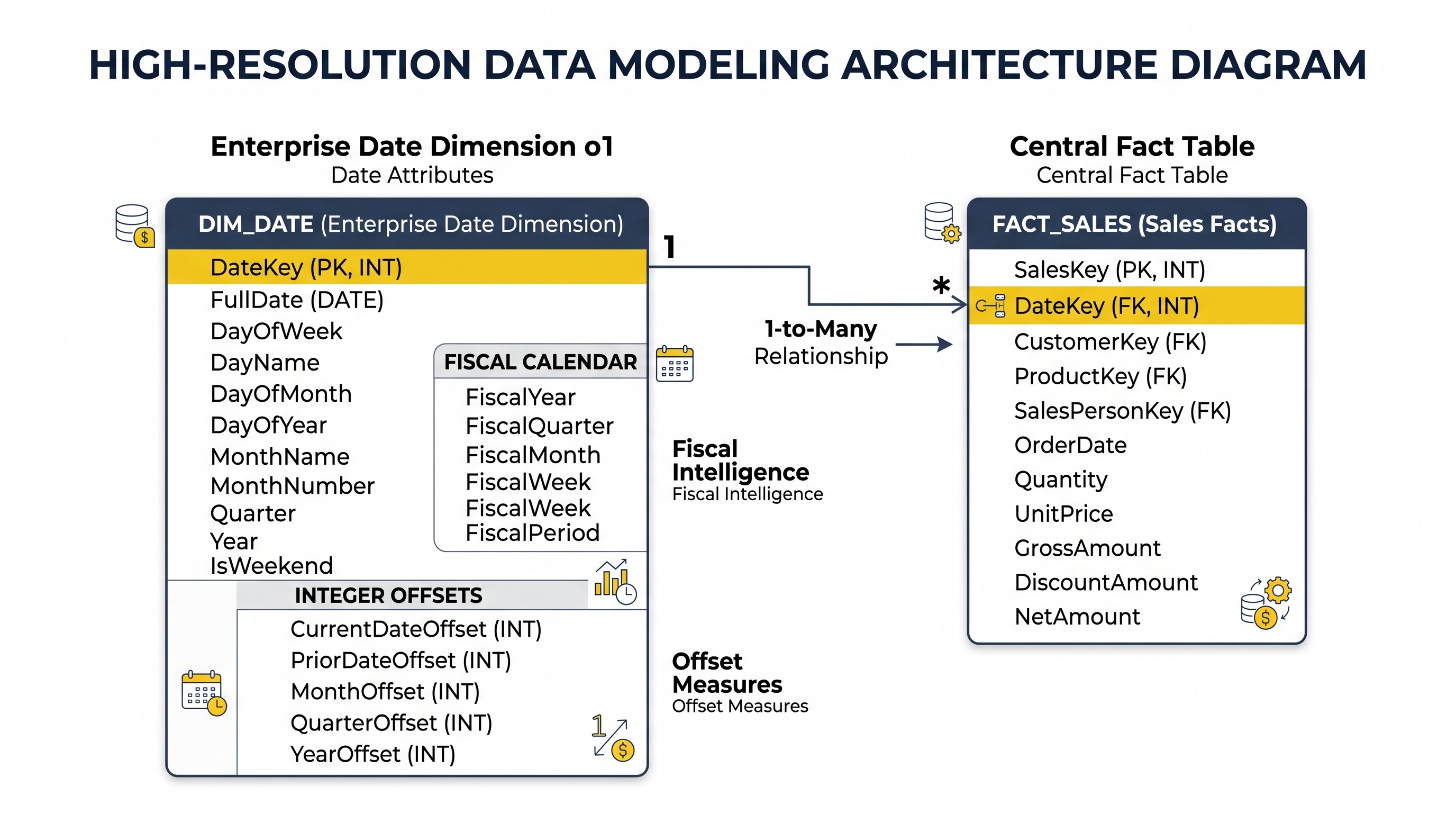
The basic requirement for performing temporal operations in a reliable manner is a Date dimension suitable for enterprise use. Thus, time-based operations in analytical systems never use transaction files to obtain time-related information. Instead, they utilize a special table created purely for calendar purposes with the only aim of acting as a source of time-related information. If there are any gaps, duplicates, or inconsistent relations in the structure of this table, all the measures derived from it will be erroneous.

The Principle of Continuity

To create a good Date table, one has to strictly adhere to the principle of continuity. It is necessary that every day in the calendar be represented in the table by a single record. There should be no missing dates no matter whether the company is working on weekends or holidays or has any planned downtime.

In situations where algorithms in time intelligence either revert the context of their filters or manipulate cumulative spans, this takes place as per the principles of date continuity. When the weekends are excluded from the calendar, the lookback over a period of thirty days will mistakenly skip some days and, thus, arrive at the incorrect calendar and destroy period-to-date aggregates.

Boundary Span and Granularity Alignment

The edges of the Date dimension must completely cover the entire time frame of all transaction fact tables. The calendar must start on or before the date of the first transaction and finish after the time of the last transaction, which can be either future plans or forecasts.

Granularity alignment is equally significant. The Date dimension needs to be designed in an atomic way of one calendar day exactly. Adding time values (hours, minutes, and seconds) to the Date dimension will negatively influence the results, lead to great cardinality growth, and thus violate the one-to-many principle needed for the standard time intelligence features. If transactional mechanisms record time with sub-day accuracy, it is necessary to separate timestamps at the level of ingestion, in order to have a Date dimension as well as a Time-of-Day dimension in the data.

Disabling Auto Date/Time and Focused Modeling

One of the weak points of corporate modeling is dependence on the more or less automated calendar features. For example, Power BI automatically creates a calendar for each of the date fields in the model. Such behavior takes more storage space, negatively affects memory usage, does not allow for synchronizing dates across tables, and makes it difficult to take a look at the overall architecture of the system.

The task of professional data modeling starts with disabling auto date-time and creating one Date dimension that can be used for all the purposes.

In this regard, it is necessary to mark this table as a Date Table in the model metadata, as well as specify a specific primary key date column with the real date data format. Marking the table as Date Table automatically tells the data storage and formula engines not to use surrogate keys and apply techniques of referential integrity and optimized filtering methods required for standard time-based calculations.

Understanding Evaluation Context in Temporal Analysis

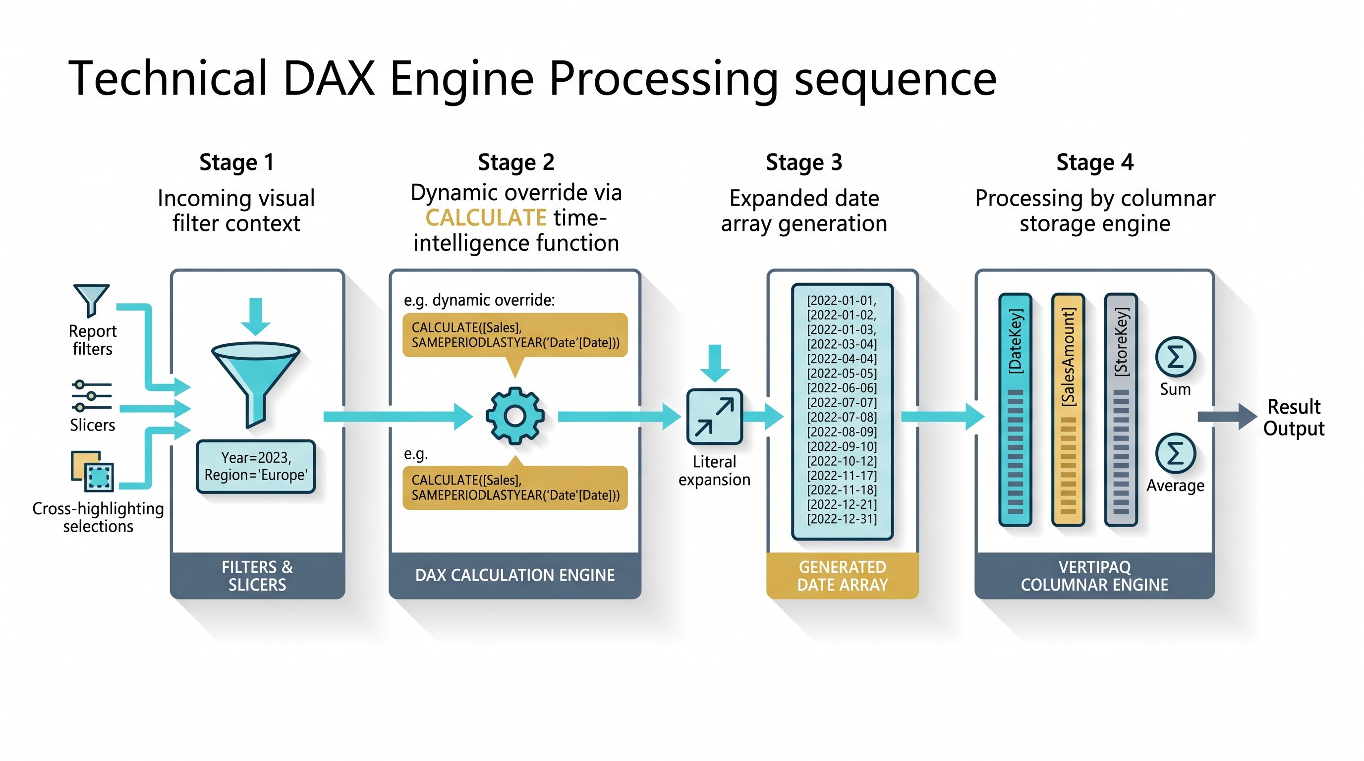
The entire essence of the success or failure of the temporal calculations relies on the understanding of the functioning of the evaluation context used by analytical engines.

Distinction Between Filter Context and Row Context

Row context operates when an engine processes a table row by row according to the values in the row. Filter context provides an overall filter for data before carrying out any aggregations. The concept of time intelligence is based on the procedure of changing the filter context in a programmatic manner.

Whenever a user selects a month in a report view, the filter context restricts the entire data model to the transactions related only to that month. When calculating the Year-to-Date aggregation, the calculations can’t just sum up the filtered transactions but must change the filter context as well. It should go back in time according to the date dimension and should populate the data with all the dates from the year in question to the current maximum date.

The Process of Context Transition

By converting row contexts to comparable filter contexts, context transition allows the analytical engine to transform row based data into well-defined filter criteria. In case of temporal calculations, context transition occurs when one does a calculation within an iterative process.

When left unregulated, such transitions can cause clashes between outer filters used by participants of operations and inner movements of dates. For example, if the participant puts a single day on the axis of the visual, the analytical engine has to figure out whether it computes the results of that particular day, the results received up to that day, or the results received on that day in comparison to the same day of the previous year.

The built-in time functions work by removing the current granular filters applied to the Date table and substituting them with a new set of filter dates which is representing the period required. In case the underlying Date table is not functioning properly or filters have been applied to calculated columns rather than to the primary Date, the analytical engine fails to update the filter context properly, which leads to empty visualization or repeated results.

Learning how context transitions work with filter propagation involves practical experience and is why power bi online training programs stress having a solid understanding of evaluation context mechanics before progressing to advanced DAX.

Compiling the Cumulative Metrics: The Year-to-Date and Quarter-to-Date Procedure

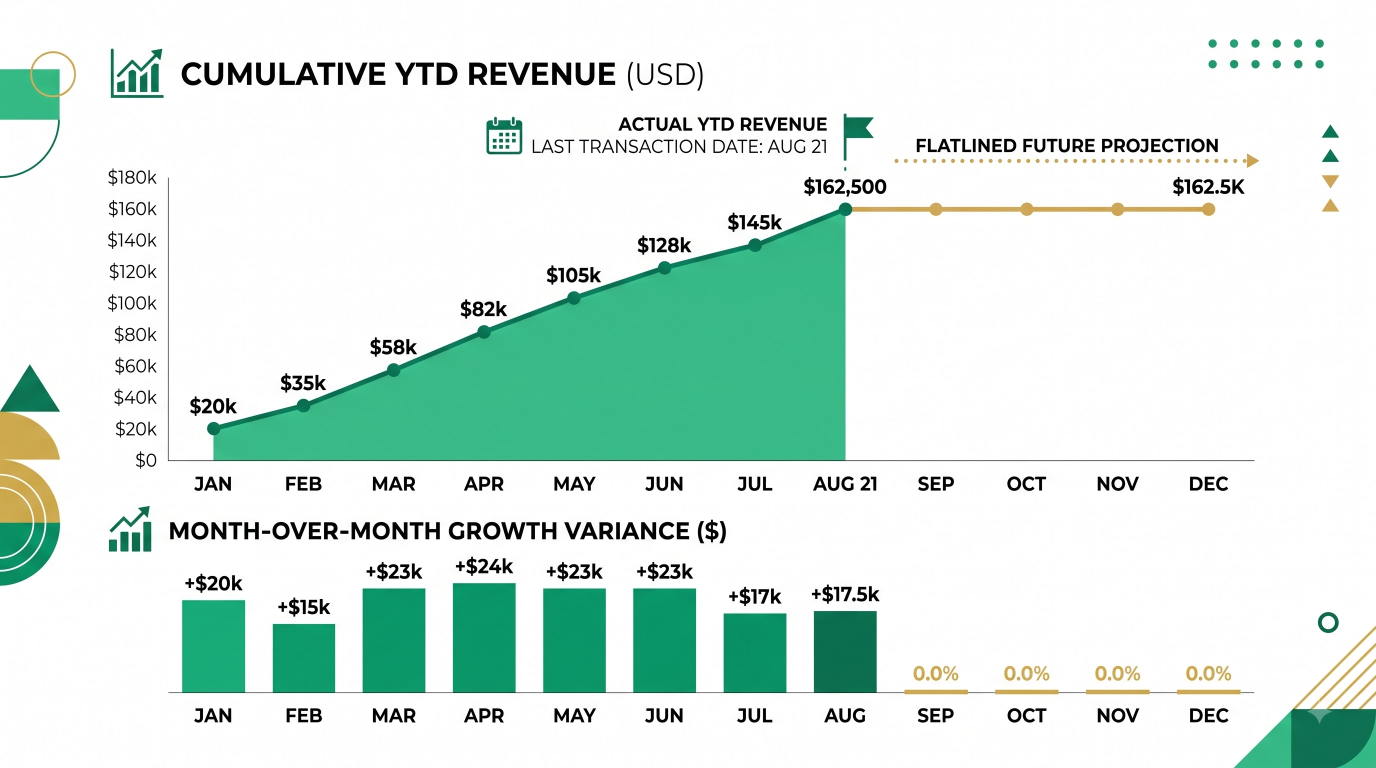
Cumulative metrics are one of the fundamentals of financial and operational reporting. Year-to-Date and Quarter-to-Date calculations derive values progressively along a specified time span, resetting back to zero once a new cycle starts.

The Basic Principle of Accumulation

The basic principle of calculating the period-to-date metric is based on finding the most recent date available in the selected time frame of the calculation and moving backwards to the first day of the specified time frame. When calculating the Year-to-Date metric, it is necessary to determine the maximum date available in the currently used visual component, find the beginning of the relevant calendar or fiscal year, and formulate an uninterrupted filter starting from that date to the maximum date.

The process is easy to follow when dealing with closed historical periods. At the same time, difficulties arise for the analysis of open periods and for reporting dates in the future.

Concerning the Future Date Flatline Issue

The problem of the future date flatline occurs in cumulative reporting. If a Date table extends to the end of the year but the data is only up to now, Year-to-Date measures display the same figure of accumulation count for every month left in the year. Consequently, there are boring horizontal lines on a line chart, and also there are repeated figures in a matrix visual.

Such a problem is resolved with the help of defensive modeling. To do so, there has to be a measure that tests if the process happens in reality. By evaluating the lowest date of the location and the greatest date of the transaction data the metric deals with empty values instead of past values.

Fiscal Calendars and Nontraditional Year Boundaries

Not every organization follows the traditional Gregorian calendar with its end of the year on December thirty-first. There are a number of businesses, government agencies, and educational organizations that comply with fiscal years, which may start on April first, July first, or October first. When calculating the cumulative amounts of the data, non-standard fiscal years must take into account the fiscal year-end boundary.

In case if there is no mention of this boundary parameter, the application will change the fiscal year boundary to December thirty-first automatically, thus making wrong calculations based on the incomplete data. As well, the Date dimension should have the relevant attributes, which describe fiscal years, fiscal quarters, and fiscal months in order to create adequate reports.

Periodic Variations Mastery: The Meaning of Month-over-Month and Growth Trends

The use of month-over-month growth rate is important for identifying new patterns, problems in processes, and work increase in relation to company divisions. In month-to-month analysis, the performance of a specific month is analyzed in comparison to the previous one, including changes in numbers and percentages.

Basics of Period Adjustment

In order to carry out the comparison of the current month against the previous one, the calculation center should take the present date range in the term of the filter being used and move it backward by one time unit. For example, if the user uses March in the system, the engine gathers all the dates throughout March, and one month is shifted back, which means that the analysis will be made covering February instead of March.

Despite the appearance of its simplicity, this mechanism frequently encounters obstacles related to data integrity.

The issue of unequal month lengths

The months of the Gregorian calendar are all composed of a different number of days. When moving a month with thirty-one days (like March) back by one month into a month where February occurs with twenty-eight or twenty-nine days, the engine must figure out how to adjust for missing days.

Standard time intelligence engines address this issue through the movement of one block of an entire month to replicate the time span of the preceding month without regard to the duration of the month in terms of days.

However, when examining data by the day, i.e. comparing the thirty-first of March with the previous month, the engine discovers a missing thirty-first for the month of February. Eventually, the engine returns an empty response for a particular day in standard cases or maps it to the last day of the target month. Data architects should ensure that regulations regarding the use of the day-by-day or monthly methodology are properly defined to avoid data presenting ungrounded interpretations of daily variations.

Removal of Division by Zero and Negative Growth Conundrums

The percentage growth calculation process can bring mathematical fallacies that should be avoided at the analysis stage. The standard formula for calculating percentage growth is the amount of difference between the present period and the preceding period divided by the preceding period.

In case the preceding period amount equals zero, standard mathematical division leads to infinite numbers and run-time errors. In case the preceding period amount is negative, which is often seen in net net, cash flow or variance amounts, standard division will give a reversed and senseless growth value.

For example, net income change from negative one hundred thousand dollars to positive fifty thousand dollars will provide a negative growth value even though there is a considerable improvement of operations.

Smart design of metrics should involve the protective formula depending on the sign and scope of the divisor amount. The formula has to either provide a blank value or an absolute value adjusted growth number without leading any visual errors or false messages.

Historical Parity - Same Time Last Year and Similar Periods

Year-On-Year analysis is the safest bet if you want to eliminate seasonal volatility. By comparing results to comparable periods from last year, one can separate real structural growth from predictable seasonal spikes such as holiday shopping or summer travel.

Differentiating Date Shifts from Similar Periods

There are two methods of making historical comparisons – date shifts or structural shifts. Date shifts take the dates used in filter context and simply shift them by the amount of one year in the past. For instance, if the user selects from January 5 to January 20, the calculation will be performed for the same period from the previous year.

Structural shifts, on the contrary, involve shifting whole time buckets. For example, if the user is examining data from a daily point of view but is doing a parallel quarter comparison, the entire parent quarter will be shifted back by one year regardless of the filter settings.

Grasping this distinction is crucial to multi-level visual hierarchies in which analysis must be able to drill down from year to quarter, month, and day with perfect data consistency without ending up with conflicting numbers.

The Mid-Month and Partial-Period Reporting Dilemma

There is one problem that can arise in Year-over-Year reporting because of the mid-month reviews. If the executive team is looking at the sales performance in the middle of the month as endorsed on the fifteenth day of that month, it can happen that the current month metric reflects sales for the first fifteen days of that month while the previous year measure reflects it for a total of thirty-one days. Therefore, the Year-over-Year comparison may show an entirely misconceiving sharp decrease in sales numbers.

In order to allow reporting to be historically consistent, one needs to implement strict methods of partial period matching. Thus, it is essential to establish the date of maximum activity in the reporting period and apply such a date offset in historical rankings as well.

In situations where the present dataset is assessed up to the fifteenth day of the current month, the earlier timeframe can only be analyzed up to the fifteenth of the year in question.

With leap years, every four years an extra day is added to the calendar so that an extra date, the February 29th, has to be analyzed.

Leap Year Adjustments

When it comes to analyzing February 29th, if we shift back this day by one year we’d reach the twenty-eighth of February of a normal year.

If we move forward from a normal year to a leap one, the date February 29th disappears and we would be able only to compare it with the previous twenty-eighth of the month if we have the corresponding necessary systems for day comparison.

Industries that depend on daily volumes like telecommunications need to take into account that there are special practices to analyze data with respect to leap years.

Custom Calendars and Unique Time Models

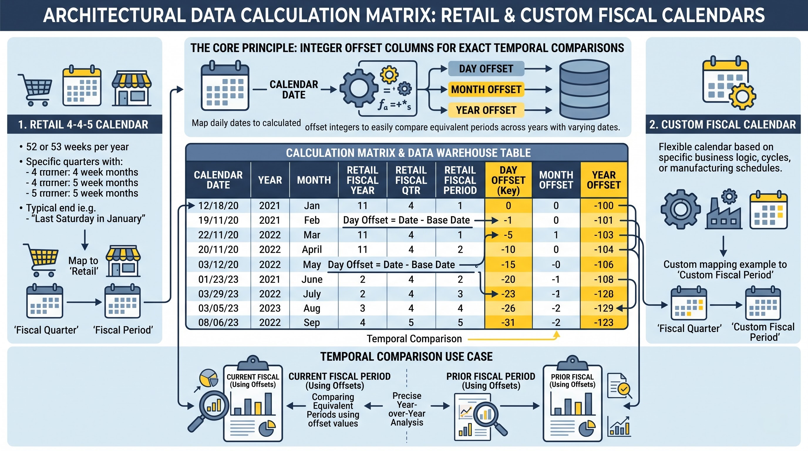
Even though standard time intelligence functions function properly according to normal Gregorian calendar rules, many areas of the economy operate outside of nine-to-five. Retail and manufacturing, consumer goods and hospitality businesses use different calendars than 4-4-5, 4-5-4, or 5-4-4 retail calendars. They also use thirteen periods and ISO weekly calendars.

Reasons Why Built-In Time Intelligence Does Not Work with Custom Calendars

Built-in time intelligence functions are programmed in a certain way, which leads them to follow standard Gregorian calendar rules. They also rely on a number of assumptions, namely that January has thirty-one days, February has twenty-eight or twenty-nine days, and the calendar year expands in time.

Within the 4-4-5 retail calendar system, the analytical year is split into four quarters, which consist of two four-week months and one five-week month. Every month starts on a particular day of the week (like Sunday) and ends on a Saturday, ensuring that every month has an exact multiple of seven days and the same number of weekends.

If you use standard Gregorian functions with the 4-4-5 retail calendar, the system will apply the Gregorian date shifts without taking into account the fact that the month has ended on the floating Saturday, therefore ruining the day-of-week correlation, and mixing trading days and non-trading days, making the comparison of retail performance meaningless.

Building an Offset-Based Date Architecture

In order to secure an unbreakable time intelligence in non-standard calendars, the data architect needs to reject the built-in Gregorian functions and utilize the offset-based calendar architecture.

In this kind of architecture, the Date dimension is complemented by columns containing sequential integers.

• Day Offset: This defines the day number in relation to the current day (i.e., zero for the current day, -1 for yesterday, and +1 for tomorrow).

• Month Offset: For each day of the month in the given fiscal or retail month, identical day numbers are assigned.

• Quarter Offset: Assigns day numbers of the quarter.

• Year Offset: Assigns day numbers of the year.

In more complicated retail cycles, the method of applying custom offset logic is an advanced technique examined in interactive power bi live training sessions, as this can enable teams to deliver custom fiscal models.

Using Offsets in Dynamic Shifts:

Integer offsets allow for the execution of complex calculations with ease. For example, in order to calculate the previous month within a 4-4-5 calendar, instead of calculating the date differences, the current Month Offset that is available in the filter context is simply checked. The value of 1 is taken away from that number in order to figure out the previous Month Offset, and therefore, all dates corresponding to the new Month Offset in the Date dimension are returned.

Calculating Year-to-Date for a custom calendar involves first determining the current Year Offset and then filtering for all days with that Year Offset while restricting the upper boundary to days where the Day Offset is less than or equal to the maximum Day Offset visible in the current selection.

This offset method is robust in all situations. It works perfectly for Gregorian calendars, 4-4-5 retail structures, ISO week systems, academic cycles, all without making any engine-specific calendar assumptions.

Managing the 53rd Week Phenomenon

A problem specific to the week and retail calendar structure is that every five to six years there is a fifty-third week. This is required to reconcile the three hundred and sixty-four day retail cycle with the astronomical solar year.

During a fifty-third week, Year-over-Year comparisons are structurally misaligned, comparing week fifty-three of this year to a nonexistent week in the prior year or rolling the entire following year out of seasonal alignment.

This is solved by an offset Date dimension which contains attributes which map special weeks for comparison. These attributes enable business analysts to decide if week fifty-three is to be compared to week fifty-two of the previous year, considered as a stand-alone non-comparable period or mapped using restated historical baseline weeks.

Conclusion: The Ground of Analytic Truth

Time intelligence is much more than a set of reporting formulas; it is the lens through which an organization measures its momentum, assesses strategic execution, and charts its future course.

To build dynamic resilient Year-to-Date, Quarter-to-Date, Month-over-Month and Same-Period-Last-Year comparisons, it is necessary to move from ad-hoc formula authoring to architectural discipline.

By anchoring analytical systems on a pristine, contiguous Date dimension, understanding the intricacies of evaluation context, adopting offset-based approaches for non-standard calendars, scaling metric architecture through calculation groups, and optimising for the underlying columnar storage engine, data experts are able to create temporal analytics that are mathematically perfect, blazingly fast, and utterly unbreakable.

In order to learn these principles using labs, examples, and business models of data, join expert power bi classes online now to boost your analytical design.