
Power BI E-Commerce Analytics: Funnels, Abandonment, LTV, and Repurchase Intervals
Last updated on Sep 23, 2026
The contemporary e-commerce environment is characterized by excessive transaction numbers, behavior as well as operational figures data. Each of the online shops produces continuous click, viewing, checkout, help task and post-purchase interaction records. However, in spite of this huge amount of information, many digital retail workers have the knowledge of gross income and advertising expenses only, without being able to determine where the losses occur.
In order to establish this connection, it is necessary to turn away from using different dashboards and independent programs. E-commerce companies usually work with disconnected reports using web website analytics to gather data about the top of the funnel, payment processors to monitor payment processes and CRM systems to store demographic information about customers and inventory systems in order to register operations after the sale.
Microsoft Power BI provides the analytical architecture that can fuse all these many forms of data into a singular machine for the purpose of understanding behavior and actions. Businesspeople will be able to turn raw event logs into useful decision-making processes through the creation of an appropriate model of the three most significant stages in the customer journey, which are drop-offs from the funnel, cumulative value over time and speed of acquisition. Business professionals wishing to create these solid models from the ground up frequently learn DAX as well as ETL processes with the help of specialized online power bi training.
This guide describes the process of structuring, modeling, analyzing, and displaying e-commerce funnel analytics in Power BI with particular emphasis on cart abandonment, customer lifetime value, and the time intervals between purchases while sticking to rigorous analytical discipline and enterprise grade architecture.
The Strategic Importance of Funnel Analytics in Today’s E-Commerce
Funnel analytics can be regarded as a simple metric of conversion ratio – the ratio of the total number of website visitors who made a purchase. Even though that conversion ratio is a good indicator of success, using it as a single metric leads to misunderstanding of the mechanisms behind it, including behavioral intentions of consumers, technical obstacles, and demand elasticity.
A modern e-commerce funnel consists of two main components:
Pre-Purchase Conversion Funnel: The sequential journey of customers who come from external traffic, discover the product, add the product to the cart, proceed to checkout, and complete the order.
Post-Purchase Retention System: The cyclic process that defines whether the first-time buyer will return for the next purchase and how much money he/she will spend in subsequent months.
Power BI’s dual domain analysis provides advantages not possible with traditional online analytics tools. While web analytics supplies accurate session metrics and earnings processes, it falters when it comes to modeling data, laying out the historical timeline of users, redistributing the analysis of historical data, or integrating with the back-end ERP systems. In turn, databases utilized in commercial and communications transactions give accurate records of financial transactions, but can’t provide the analytics of website sessions.
Power BI unites the two domains, applying its column-wise VertiPaq technology. By importing various records, including granular data of clicks and confirmed data on transactions, experts are able to assess the financial effect through the used behavior matrix.
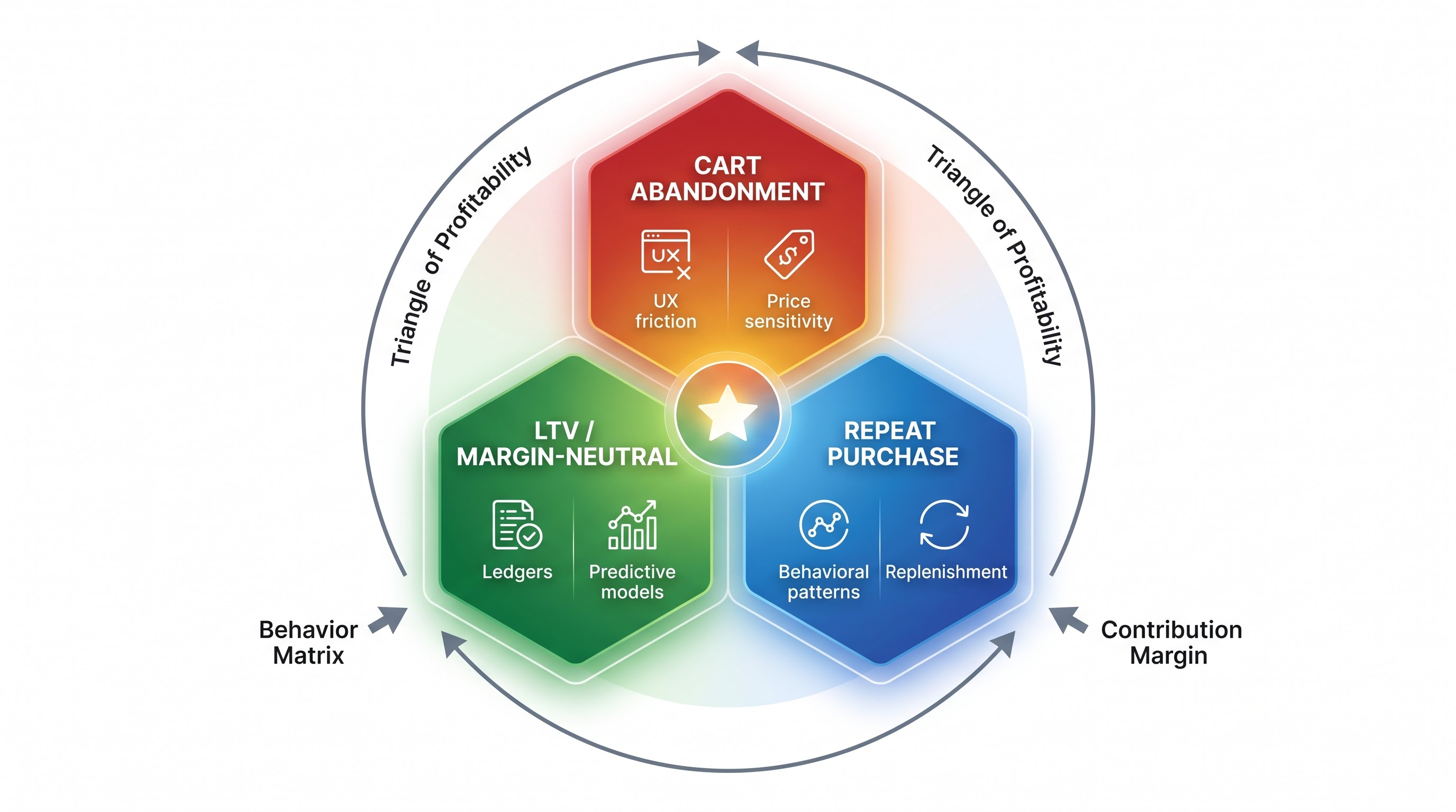
There are three fundamental metrics in this model—the abandonment of shopping carts, customer net worth, and the cycle of repeat purchases—which works in collaboration, forming the triangle of profitability.
Abandonment of shopping carts gives a window into micro-friction, sensitivity to price, and UX bottlenecks that stand in the way of revenue capture.
Frequency of repeat purchases shows behavioral patterns, replenishment cycles, and stickiness of a brand.
Customer lifetime value puts acquisition cost into context that shows how much capital one can allocate toward acquiring customers in various categories.
When these three dimensions are captured within an enterprise semantic model, executive teams can clearly see the effectiveness of changes made at the upstream side of the checkout design on long-term customer profitability.
Designing the Basic Data Model in Power BI
The first thing to consider before setting up any visualizations or performing evaluations is the development of a durable data model. An incorrectly formed schema necessitates complex analytical expressions, makes report generation much slower and creates excessive memory consumption.
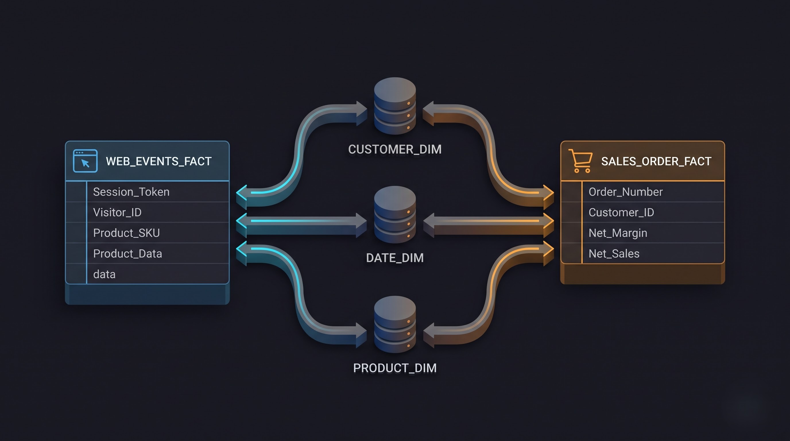
In order to enable the analysis of both funnel activity at the session level and dynamics of customer indicators without compromising the level of efficiency, the semantic model must adhere to a rigid dimensional modeling theory whereby the star schema should prevail. There is a mistake capitalized on in e-commerce sales analytics because the teams try to process session data and multi-year sales history in a single flat-file format with millions of duplicated rows in high-cardinality attributes, which leads to malfunctioning of the engine compression algorithms.
The right Power BI structure ensures that analytics is divided into different fact tables and supported with several dimension tables.
Multi-Fact Architecture
An optimal eCommerce architecture consists of at least two significant fact casting tables at varying granularity levels.
The Web Events Fact Table (Session Grain): In this table, each particular interaction during the conversion journey is recorded. Each row comprises a particular interaction by the user, which can include a page viewed, a category searched, a product detail page viewed, adding item in the cart, cart viewed, starting the checkout process, completing payment, and the transaction confirmed. This means that a particular event is recorded for each timestamp and visitor.
The Sales Order Fact Table (Transaction Grain): The commercial transactions that have been processed and verified through the order management or the enterprise database are captured in this table. The fact table includes specific items that are part of a single order, meaning that specific details about that order are captured in each row, which includes the order number, product number, quantity, price of each unit, discounts, taxes, shipping costs, as well as returns status.
Using different tables for clickstream data versus finalized orders creates a separation that prevents clickstream data from overwhelming financial reports.
Core Conformed Dimensions
These two data cubes are associated with multiple shared dimensions that facilitate the linking of different facts for filtering and analysis of related data:
Customer Dimension: This dimension has one record per customer, and carries relatively stable demographic measures, main delivery places, lead sources for acquisition, first date of some dealings with the customer, and the status of the account.
Date Dimension: This dimension consists of a highly elaborate calendar, which has been marked as the main date dimension table within the Power BI that can represent the standard calendar hierarchy, financial calendar, day-of-week classifiers, and holiday identification.
Product Dimension: This dimension contains definition for product hierarchy which involves SKU, parent products, product brands, cost data, margins, launch period.
Traffic and Marketing Dimension: This dimension provides classification of incoming acquisition channels, including sources of the campaign, methods of promotion, creative styles, referring sites, and identifiers for the platforms.
Structure of Relationships and Their Direction
In order to keep the report consistent and free from confusion:
Every relation between the dimensions and the facts has to be one-sided.
The cross filtering should always be in one direction from the dimension tables to the fact tables. Bidirectional filtering must be avoided because of its potential burden on the planning of queries and unpredictability of the calculations involved during complicated time-based calculations.
Quite a number of foreign keys having a big number of records should be studied carefully, as it is essential to achieve maximum compression with the help of the VertiPaq technology. If customer identifiers that involve either text or session tokens are utilized, it is suggested that they be encoded into numeric format when preparing the data for actual production. Since processes like VertiPaq compressions, unidirectional relationships, and high-cardinality keys are rather complex, attending extensive power bi classes online will give analysts an opportunity to obtain practical experience in the design of effective star schemas.
Analyzing Cart Abandonment: A Decline in Sales
Cart abandonment refers to simply a formula in business; the formula used to calculate abandonment is the number of times the customer added an item to the cart but did not buy something, divided by the total number of cart sessions. However, this would not be a true picture since analyzing it as a static metric would not allow doing anything about it.
In order to make useful conclusions about cart abandonment using Power BI, it is important for analysts to understand the difference between abandonment due to customer’s intention and abandonment due to mechanical processes, check how abandonment occurs at each step, and evaluate financial losses resulting from abandoned pipelines.
Phases of Checkout Losses
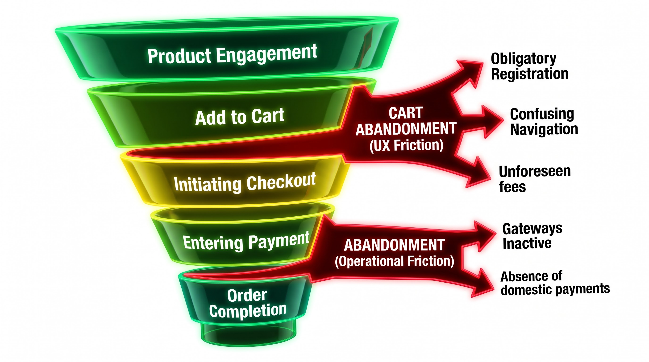
An elaborate e-commerce conversion model identifies separate points of sales cycle.
Product Engagement: The guest engages with product pages, reads specs, and checks feedback from previous customers.
Add to Cart: The buyer shows intent to purchase by adding an item into their basket.
Cart Viewing: The buyer checks his/her selected products, looks at the total amount, and decides what to do next.
Initiating Checkout: The buyer stops browsing and starts entering necessary information for shipping and identifying purposes.
Entering Payment: The buyer enters billing details, is confronted with the final estimate of shipping fees and taxes, and gets to the final confirmation page.
Order Completion: The payment processor confirms the payment and generates a code for the order, so a customer reaches the order confirmation page.
In Power BI, all steps in this sequence are monitored through the calculation of survival rates from step to step and funnel component progression.
When the greatest decrease happens between the cart review and payment initiation, the conflict typically arises from strategic reasons: unforeseen fundamental shipping fees, obligatory user registration requests, or perplexing navigation patterns. When the drop occurs during payment combination and finalization, the issue is often operational: inactive gateways, surprising additional charges, absence of desirable domestic payment options, or puzzled multi-factor authentication circles.
Analyzing Cart Abandonment by Product and Target Segments
Power BI gives organizations the ability to break down the cross-section rate of cart abandonment into various dimensional criteria. Instead of just settling for the industry standard abandonment number equal to seventy percent, the enterprise report must raise more sophisticated diagnostic issues:
Elasticity by Product Category: are high-price electronics being abandoned more often than low-priced accessories? In the majority of cases expensive goods have a prolonged period of decision-making in which clients see the cart as a sort of temporary wishlist.
Traffic Quality and Site Usability: Do visitors from paid social channels drop-off at double the rate of those from organic search? Paid social traffic typically leads to impulsive clicks by motivated mobile users who have trouble filling out mobile forms. Reviewing abandonment by acquisition source and device operating system can efficiently allocate engineering resources.
Shipping Geography Impact: Do customers from certain areas abandon their cart when they see delivery times or extra delivery fees? Filtering abandoned carts by geography helps pinpoint regions where shipping processes become roadblocks to completing sales.
Quantifying Inaccessible Funds and Recovery Potential
Beyond just percentage metrics, Power BI should provide details of the monetary amount tied in abandoned carts.
By measuring the total retail value of abandoned products, the business is able to estimate losses incurred due to abandoned carts but an advanced analytical dashboard takes the analysis a step further by determining the realistic limits of what can actually be recovered from abandoned carts.
Utilizing the information gleaned from past user behavior regarding forsaken carts, such as whether or not a consumer is an established loyalty member or new user, businesses are able to easily determine what is known as an adjusted amount available for consideration of conversion. This figure provides the lifecycle marketing teams with an objective measurement that can be used as a reference when evaluating effectiveness of automated abandonment recovery emails, SMS reminders, and personalized retargeting campaigns.
LTV Modeling: From Getting Customers to Maintaining Them
While the review of shopping cart abandonment contributes to the efficiency of short-term sales, the Customer Lifetime Value (LTV) determines the long-term allocation of funds. The LTV means the whole sum of money that a client gives to the organization during the whole time of his contractual relationship with the customer.
In the absence of correct LTV modeling in Power BI, organizations easily fall into the perilous strategic traps. For example, they may waste extra money on clients who make the first purchases but never return again, or alternatively they may set artificially low spending limits for client groups that may seem expensive, but provide stable margins in the future.
Comparing Historical and Predictive LTV Techniques
In the case of Power BI, one can take the advantage of two alternative techniques to measure LTV:
Historical Realized LTV: It refers to determining the total money gained by particular historical cohorts over respective periods of time (i.e., in the last 12 months, 24 months, or 36 months). The method is based on reliable ledger entries, that is why it gives good insights from the point of view of the history of customer behavior, which is useful to assess how businesses performed over time.
Predictive Modeled LTV: It is concerned with anticipation of various amounts based on the aspect of previous transactions, respective probabilities of retention, etc. The calculations are usually done in special statistical systems and then introduced into the Power BI system for any visualization according to the collected data.
The majority of reporting capabilities offered by Power BI is founded on the historical method of computation of cohort lifetime value (LTV). To become proficient in the advanced time-intelligence DAX functionalities necessary for cohort tenure modeling, many developers utilize organized power bi online training that include real-life scenarios of business retailers.
Most of the reporting functions of Power BI are based on the historical approach of cohorts LTV calculations.
Customer Lifetime Value Architecture Based on Cohorts
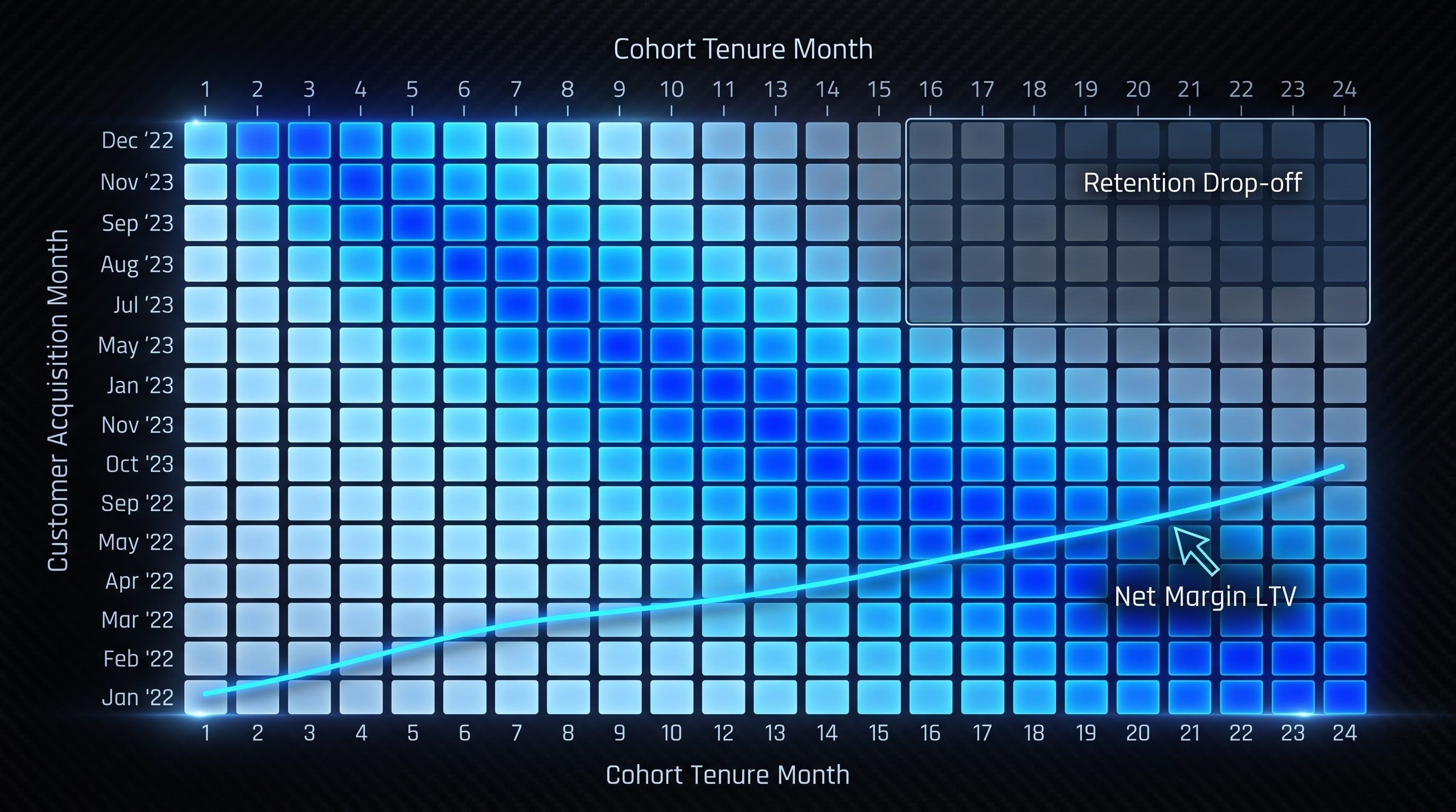
When utilizing Power BI to establish customer lifetime value, the best methodology is by creating cohorts based on customer acquisition. A cohort is defined as the month or quarter in which the customer made their first valid purchase.
Determining the LTV based on the unsegregated and aggregate analyses conceals trends. Take for example the scenario where total sales increase while retaining customers is on the decline; metrics calculated in an aggregated manner may conceal the falling off of numbers provided that acquisition volume is on the rise.
When customers are linked to the acquisition date, the revenue of the organizations can be monitored along the stages of customer life cycle:
Zero Month: Revenue earned in the month.
The First Month: Revenue generated by the cohort in the second month.
The Second, Third, Twelfth month and so on: Revenue over time.
Cumulative margin of a cohort can be tracked in Power BI, by dividing the cumulative margin value over the first cohort number.
In this net margin, comparisons can be made among different cohorts like:
Comparing the value accumulation of the cohort that joined over the holiday season to that of the cohort that joined during the spring launch is also possible.
Is any improvement noted with current strategies that have enhanced value accumulation when compared with older strategies?
Net Margin and Gross Revenue LTV
If any reports are prepared on the e-commerce industry to develop LTV models, the revenue-based LTV will paint a rosy picture.
For a valid LTV model, it is imperative to focus on Contribution Margin LTV.
The accurate margin per customer can be calculated using the following method:
It takes the total production process or cost of manufacture into consideration.
All costs related to transport, packing, and shipping are included.
Costs paid through various payment gateways are included in calculations of direct sales.
All discounts given to customers are included in the calculations.
When executive teams contemplate LTV based on contribution margin, the strategic narratives become completely different. Some customer segments that seem very lucrative under revenue assessment are projected into margin neutral or margin negative categories. In contrast, smaller segments with high full-price transaction rates that seldom return any purchases show up as the strong financial backbone of the business.
Achieving balance between LTV and CAC
LTV becomes much more meaningful when considered along with customer acquisition costs.
By factoring in the blended and paid marketing spend from the traffic and marketing aspects, Power BI is able to gauge the ratio of LTV to CAC among mature customer cohorts.
Monitoring the period necessary for achieving profitability by a cohort enables managers in finance and marketing departments to make data-driven decisions regarding budgeting for performance marketing, investments in retention and stock management.
Conclusions: Strategic Takeaways
The transformation of raw data related to e-commerce into information useful for making business decisions requires overcoming the boundary of simple conversions and linear accounting of transactions. By building a star schema in Power BI that ties session-level events to historical customer data, today’s online businesses are able to gain a holistic view of consumer behavior.
By calculating Customer Lifetime Value on a cohort by cohort basis—based on the truth of the contribution margin rather than inflated top-line sales—management gets an objective starting point to analyze marketing expenses, improve working capital, and safeguard company margins.
Understanding the repeat purchase rate helps to determine consumption processes across various product categories.
When these three analytical foundations converge on the flexible and smoothly functioning Power BI framework, the analytical department stops at being just a reporting function of past performances, but gets transformed into an important facilitator of those processes aimed at improvement of conversion rates and retention of customers.
If you are interested in moving to the next level of analytics, switching from just dashboard reporting to creating the entire data architecture required for commercial analytics, check out the top best online power bi course launched by OnlineITGuru and start learning.